- Published on
API Sneak Peek: Train an Object Detection Model on Pascal VOC 2007 using KerasCV
- Authors

- Name
- Luke Wood
⛔ KerasCV's object detection API is now launched! ⛔
⚠️ Instead of reading this post, visit the linked tutorial! ⚠️
Overview
KerasCV offers a complete set of APIs to allow you to train your own state-of-the-art, production-grade object detection model. These APIs include object detection specific data augmentation techniques, models, and COCO metrics.
import sys

import matplotlib.pyplot as plt
import tensorflow as tf
import tensorflow_datasets as tfds
import wandb
from absl import flags
from tensorflow import keras
from tensorflow.keras import callbacks as callbacks_lib
from tensorflow.keras import optimizers

import keras_cv
from keras_cv.data import bounding_box
Data loading
In this guide, we use the data-loading function: keras_cv.loaders.pascal_voc.load(). KerasCV supports a bounding_box_format argument in all components that process bounding boxes. To match the KerasCV API style, it is recommended that when writing a custom data loader, you also support a bounding_box_format argument. This makes it clear to those invoking your data loader what format the bounding boxes are in. For example:
train_ds, ds_info = keras_cv.loaders.pascal_voc.load(split='train', bounding_box_format='xywh', batch_size=8)
Clearly yields bounding boxes in the format xywh. You can read more about KerasCV bounding box formats in the API docs. Our data comesloaded into the format {"images": images, "bounding_boxes": bounding_boxes}. This format is supported in all KerasCV preprocessing components. Lets load some data and verify that our data looks as we expect it to.
dataset, _ = keras_cv.loaders.pascal_voc.load(
    split="train", bounding_box_format="xywh", batch_size=9
)

def visualize_dataset(dataset, bounding_box_format):
    color = tf.constant(((255.0, 0, 0),))
    plt.figure(figsize=(10, 10))
    iterator = iter(dataset)
    for i in range(9):
        example = next(iterator)
        images, boxes = example["images"], example["bounding_boxes"]
        boxes = keras_cv.data.bounding_box.convert_format(
            boxes, source=bounding_box_format, target="rel_yxyx", images=images
        )
        boxes = boxes.to_tensor(default_value=-1)
        plotted_images = tf.image.draw_bounding_boxes(images, boxes[..., :4], color)
        plt.subplot(9 // 3, 9 // 3, i + 1)
        plt.imshow(plotted_images[0].numpy().astype("uint8"))
        plt.axis("off")
    plt.show()


visualize_dataset(dataset, bounding_box_format="xywh")
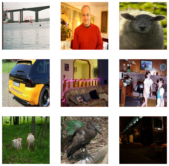
Looks like everything is structured as expected. Now we can move on to constructing our data augmentation pipeline.
Data augmentation
One of the most labor-intensive tasks when constructing object detection pipeliens is data augmentation. Image augmentation techniques must be aware of the underlying bounding boxes, and must update them accordingly.
Luckily, KerasCV natively supports bounding box augmentation with its extensive library of data augmentation layers. The code below loads the Pascal VOC dataset, and performs on-the-fly bounding box friendly data augmentation inside of a tf.data pipeline.
# train_ds is batched as a (images, bounding_boxes) tuple
# bounding_boxes are ragged
train_ds = keras_cv.loaders.pascal_voc.load(bounding_box_format="xywh", split="train", batch_size=2)
val_ds = keras_cv.loaders.pascal_voc.load(bounding_box_format="xywh", split="validation", batch_size=2)

augmentation_layers = [
    keras_cv.layers.RandomShear(x_factor=0.1, bounding_box_format='xywh'),
    # TODO(lukewood): add color jitter and others
]


def augment(sample):
    for layer in augmentation_layers:
        sample = layer(sample)
    return sample


train_ds = train_ds.map(augment, num_parallel_calls=tf.data.AUTOTUNE)
visualize_dataset(train_ds, bounding_box_format="xywh")
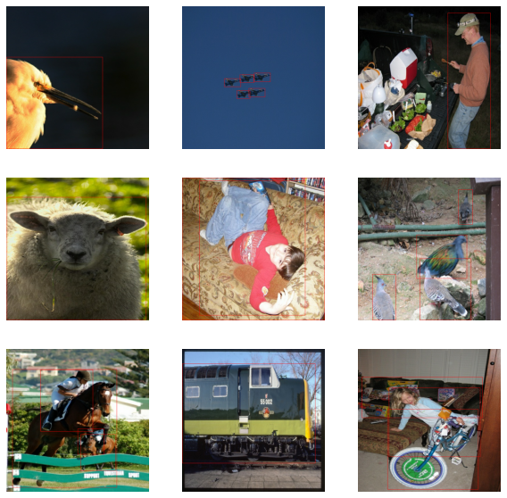
Great! We now have a bounding box friendly augmentation pipeline.
Next, let's unpackage our inputs from the preprocessing dictionary, and prepare to feed the inputs into our model.
def unpackage_dict(inputs):
    return inputs["images"], inputs["bounding_boxes"]


train_ds = train_ds.map(unpackage_dict, num_parallel_calls=tf.data.AUTOTUNE)
val_ds = val_ds.map(unpackage_dict, num_parallel_calls=tf.data.AUTOTUNE)

train_ds = train_ds.prefetch(tf.data.AUTOTUNE)
val_ds = val_ds.prefetch(tf.data.AUTOTUNE)
Our data pipeline is now complete. We can now move on to model creation and training.
Model creation
We'll use the KerasCV API to construct a RetinaNet model. In this tutorial we use a pretrained ResNet50 backbone using weights. In order to perform fine-tuning, we freeze the backbone before training. When include_rescaling=True is set, inputs to the model are expected to be in the range [0, 255].
model = keras_cv.models.RetinaNet(
    classes=20,
    bounding_box_format="xywh",
    backbone="resnet50",
    backbone_weights="imagenet",
    include_rescaling=True,
)
model.backbone.trainable = False
That is all it takes to construct a KerasCV RetinaNet. The RetinaNet accepts tuples of dense image Tensors and ragged bounding box Tensors to fit() and train_on_batch() This matches what we have constructed in our input pipeline above.
The RetinaNet call() method outputs two values: training targets and inference targets. In this guide, we are primarily concerned with the inference targets. Internally, the training targets are used by keras_cv.losses.ObjectDetectionLoss() to train the network.
Optimizer
For training, we use a SGD optimizer with a piece-wise learning rate schedule consisting of a warm up followed by a ramp up, then a ramp. Below, we construct this using a keras.optimizers.schedules.PiecewiseConstantDecay schedule.
learning_rates = [2.5e-06, 0.000625, 0.00125, 0.0025, 0.00025, 2.5e-05]
learning_rate_boundaries = [125, 250, 500, 240000, 360000]
learning_rate_fn = optimizers.schedules.PiecewiseConstantDecay(
    boundaries=learning_rate_boundaries, values=learning_rates
)

optimizer = optimizers.SGD(
    learning_rate=learning_rate_fn, momentum=0.9, global_clipnorm=10.0
)
COCO metrics monitoring
KerasCV offers a suite of in-graph COCO metrics that support batch-wise evaluation. More information on these metrics is available in:
- Efficient Graph-Friendly COCO Metric Computation for Train-Time Model Evaluation
- Using KerasCV COCO Metrics
Lets construct two COCO metrics, an instance of keras_cv.metrics.COCOMeanAveragePrecision with the parameterization to match the standard COCO Mean Average Precision metric, and keras_cv.metrics.COCORecall parameterized to match the standard COCO Recall metric.
metrics = [
    keras_cv.metrics.COCOMeanAveragePrecision(
        class_ids=range(20),
        bounding_box_format="xywh",
        name="Mean Average Precision",
    ),
    keras_cv.metrics.COCORecall(
        class_ids=range(20),
        bounding_box_format="xywh",
        max_detections=100,
        name="Recall",
    ),
]
Training our model
All that is left to do is train our model. KerasCV object detection models follow the standard Keras workflow, leveraging compile() and fit().
Let's compile our model:
loss = keras_cv.losses.ObjectDetectionLoss(
    classes=20,
    classification_loss=keras_cv.losses.FocalLoss(from_logits=True, reduction="none"),
    box_loss=keras_cv.losses.SmoothL1Loss(l1_cutoff=1.0, reduction="none"),
    reduction="auto",
)

model.compile(
    loss=loss,
    optimizer=optimizer,
    metrics=metrics,
)
All that is left to do is construct some callbacks:
callbacks = [
    callbacks_lib.TensorBoard(log_dir="logs"),
    callbacks_lib.EarlyStopping(patience=30),
]
And run model.fit()!
model.fit(
    train_ds,
    validation_data=val_ds,
    epochs=1,
    callbacks=callbacks,
    # single step epochs for demonstrative purposes
    steps_per_epoch=1,
    validation_steps=1,
)
outputs:
1/1 [==============================] - 16s 16s/step - loss: 3.4917 - Mean Average Precision: 0.0000e+00 - Recall: 0.0000e+00 - val_loss: 3.8008 - val_Mean Average Precision: 0.0000e+00 - val_Recall: 0.0000e+00

<keras.callbacks.History at 0x13bd1e550>
Results and conclusions
The new KerasCV object detection API will make it easy to construct state-of-the-art object detection pipelines. All of the KerasCV object detection components can be used independently, but also have deep integration with each other With KerasCV, bounding box augmentation, train-time COCO metrics evaluation, and more, are all made simple and consistent.
KerasCV offers train time COCO metrics, as discussed in Efficient Graph-Friendly COCO Metric Computation for Train-Time Model Evaluation (Luke Wood & Francois Chollet). These metrics are evaluated at train time, and can be used like any other train time Keras metric. This includes exportation to the experiment tracking framework of your choice such as Weights and Biases.